


MATLAB Simulation of Current Harmonic Mitigation in Grid Tied Solar PV System

MATLAB Simulation of Current Harmonic Mitigation in Grid Tied Solar PV System
𝐈𝐧𝐭𝐫𝐨𝐝𝐮𝐜𝐭𝐢𝐨𝐧
Current harmonics are one of the major power-quality problems in grid-connected renewable energy systems. When a nonlinear load, such as a rectifier-fed RL load, is connected at the point of common coupling, the load current becomes highly distorted and introduces harmonics into the grid.
Current Harmonic Mitigation in Grid Tied Solar PV System
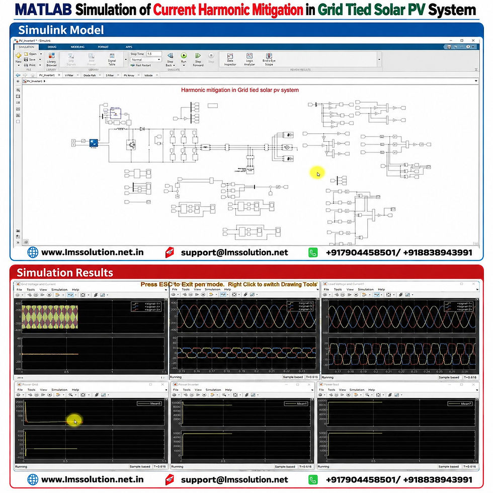
In this MATLAB/Simulink model, Current Harmonic Mitigation in a Grid-Tied Solar PV System is achieved using an Active Current Coefficient Control technique.
The proposed system performs multiple functions simultaneously:
Extracts maximum available solar PV power.
Maintains good grid-current quality.
Compensates load harmonic current.
Supplies load reactive power.
Controls the DC-link voltage.
Transfers excess PV power to the utility grid.
Operates without conventional PLL-based synchronization.
Maintains satisfactory operation during grid-voltage distortion.
Handles voltage sag and swell conditions.
The simulation is useful for students, researchers, and engineers studying solar PV integration, harmonic compensation, active power filtering, power-quality improvement, and grid-connected inverter control.
𝐒𝐲𝐬𝐭𝐞𝐦 𝐎𝐯𝐞𝐫𝐯𝐢𝐞𝐰
The complete system consists of:
Solar PV array
Boost converter
Maximum Power Point Tracking controller
DC-link capacitor
Three-phase Voltage Source Converter
Coupling inductor
Utility grid
Nonlinear load
Grid and load voltage/current measurement
Active Current Coefficient controller
Unit-vector synchronization
DC-link voltage controller
Hysteresis current controller
Main Power Flow
Solar PV → Boost Converter → DC Link → Voltage Source Converter → AC Bus → Load / Grid
The nonlinear load is connected between the PV inverter and utility grid and creates a distorted load-current waveform.
The inverter is therefore controlled not only for solar power transfer but also for harmonic and reactive-power compensation.
𝐏𝐕 𝐀𝐫𝐫𝐚𝐲 𝐏𝐚𝐫𝐚𝐦𝐞𝐭𝐞𝐫𝐬
Parameter | Value |
PV modules connected in series | 7 |
Parallel strings | 12 |
Total number of modules | 84 |
Single-module rating | 315 W |
Voltage at maximum power point | 54.7 V |
Current at maximum power point | 5.76 A |
Approximate array rated power | 26.46 kW |
PV temperature used in testing | 25°C |
PV Operating Conditions
Solar Irradiance | Approx. PV Power | Operating Observation |
0 W/m² | 0 kW | No solar generation |
100 W/m² | 2.49 kW | Low-generation condition |
400 W/m² | Around 9–9.5 kW | PV supplies major load power |
1000 W/m² | Around 26.47 kW | High PV generation and grid export |
At 1000 W/m², the PV array operates close to its maximum rated power.
𝐁𝐨𝐨𝐬𝐭 𝐂𝐨𝐧𝐯𝐞𝐫𝐭𝐞𝐫 𝐚𝐧𝐝 𝐌𝐏𝐏𝐓 𝐂𝐨𝐧𝐭𝐫𝐨𝐥
The solar PV array is connected to the common DC link through a DC–DC boost converter.
The boost converter performs two important functions:
Raises the PV-side voltage to the required DC-link level.
Forces the PV array to operate near its maximum power point.
MPPT Inputs
The MPPT controller receives:
PV voltage
PV current
The controller continuously observes changes in PV operating conditions and modifies the converter duty cycle.
The generated duty cycle is applied to the boost-converter IGBT through a PWM generator.
This enables maximum available solar energy to be extracted during changes in irradiance.
𝐍𝐨𝐧𝐥𝐢𝐧𝐞𝐚𝐫 𝐋𝐨𝐚𝐝 𝐚𝐧𝐝 𝐇𝐚𝐫𝐦𝐨𝐧𝐢𝐜 𝐏𝐫𝐨𝐛𝐥𝐞𝐦
The system uses a nonlinear load based on a rectifier with an RL load.
Because of the switching and rectification process:
Load current is not sinusoidal.
Significant current harmonics are generated.
Grid-current quality can deteriorate.
Other equipment connected to the same AC network may also be affected.
The uncompensated current Total Harmonic Distortion is approximately:
Condition | Current THD |
Nonlinear load without effective compensation | Around 22.22% |
Desired grid-current condition | Harmonic content significantly reduced |
Since the nonlinear-load current distortion is much higher than the commonly targeted 5% harmonic level, an active compensation method is required.
𝐂𝐨𝐧𝐭𝐫𝐨𝐥 𝐒𝐭𝐫𝐚𝐭𝐞𝐠𝐲
The main control technique used in this model is Active Current Coefficient Control.
Its objective is to determine the fundamental active component required from the source and generate the appropriate compensation-current reference for the inverter.
The control structure contains the following major stages.
1. Grid-Voltage Measurement
The three-phase grid voltages are measured.
The controller processes the measured voltages to obtain suitable phase quantities for synchronization and reference-current generation.
2. Stationary-Frame Processing
The grid-voltage information is transformed into stationary reference-frame components.
This simplifies voltage processing and assists in obtaining the fundamental voltage information.
3. Band-Pass Filtering
The voltage signals are processed through filtering stages.
The main purpose is to retain the required fundamental-frequency information while reducing unwanted frequency components.
4. Unit-Vector Generation
Three unit vectors are generated for phases A, B, and C.
These unit vectors provide synchronization information for generating balanced three-phase current references.
𝐏𝐋𝐋-𝐅𝐫𝐞𝐞 𝐒𝐲𝐧𝐜𝐡𝐫𝐨𝐧𝐢𝐳𝐚𝐭𝐢𝐨𝐧
An important feature of the model is that conventional Phase-Locked Loop synchronization is not required for the main reference-current generation process.
Instead, synchronization is obtained using a unit-vector-based approach derived from the processed grid-voltage signals.
Advantages include:
Reduced dependence on a conventional PLL.
Direct generation of three-phase synchronizing templates.
Suitable operation for current-reference generation.
Good compatibility with active-current-coefficient control.
𝐀𝐜𝐭𝐢𝐯𝐞 𝐂𝐮𝐫𝐫𝐞𝐧𝐭 𝐂𝐨𝐞𝐟𝐟𝐢𝐜𝐢𝐞𝐧𝐭 𝐂𝐚𝐥𝐜𝐮𝐥𝐚𝐭𝐢𝐨𝐧
The three nonlinear load currents are continuously measured.
For every phase, the controller evaluates the active-current contribution using:
Load-current information
Corresponding unit vector
Averaging/integration operations
Separate active current coefficients are determined for:
Phase A
Phase B
Phase C
The three coefficients are then combined to obtain an average active-current coefficient representing the fundamental active current required by the load.
This is the key information used to separate the required source-current component from the unwanted harmonic and reactive components.
𝐃𝐂-𝐋𝐢𝐧𝐤 𝐕𝐨𝐥𝐭𝐚𝐠𝐞 𝐂𝐨𝐧𝐭𝐫𝐨𝐥
The DC-link voltage is continuously monitored.
Parameter | Value |
DC-link reference voltage | 735 V |
The measured DC-link voltage is compared with the reference value.
The resulting error is processed through a controller to determine the additional active-current component needed for:
Maintaining DC-link voltage
Compensating inverter losses
Maintaining stable converter operation
The resulting DC-side current demand is combined with the active-current requirement calculated from the load.
𝐑𝐞𝐟𝐞𝐫𝐞𝐧𝐜𝐞 𝐂𝐮𝐫𝐫𝐞𝐧𝐭 𝐆𝐞𝐧𝐞𝐫𝐚𝐭𝐢𝐨𝐧
After calculating the total current requirement, the controller converts it into three-phase AC reference currents using the unit vectors.
The generated reference currents represent the desired grid-current waveform.
The control objective is to force the utility-grid current to become:
Sinusoidal
Balanced
Low in harmonic content
Close to unity power factor
𝐇𝐲𝐬𝐭𝐞𝐫𝐞𝐬𝐢𝐬 𝐂𝐮𝐫𝐫𝐞𝐧𝐭 𝐂𝐨𝐧𝐭𝐫𝐨𝐥
The reference currents are compared with the measured source currents.
A hysteresis current controller generates inverter switching pulses according to the current error.
Three primary switching signals are produced and complementary signals are generated for the remaining inverter switches.
As a result, the Voltage Source Converter injects the required compensation current into the AC bus.
𝐖𝐨𝐫𝐤𝐢𝐧𝐠 𝐏𝐫𝐨𝐜𝐞𝐬𝐬
The overall operation can be summarized as follows:
The PV array generates DC power according to irradiance and temperature.
The MPPT controller extracts maximum available PV power.
The boost converter transfers this power to the DC link.
The nonlinear load draws distorted current.
The controller measures grid voltage and nonlinear-load current.
Unit vectors are generated from the grid voltage.
Active load-current coefficients are calculated.
DC-link voltage regulation determines the converter loss component.
Three-phase reference source currents are generated.
The hysteresis controller generates inverter gate pulses.
The inverter injects the required compensating current.
Load harmonics and reactive-current requirements are supplied by the inverter.
The grid current remains approximately sinusoidal.
Available PV real power is supplied to the load.
Excess PV power is exported to the utility grid.
𝐒𝐢𝐦𝐮𝐥𝐚𝐭𝐢𝐨𝐧 𝐓𝐞𝐬𝐭 𝐂𝐨𝐧𝐝𝐢𝐭𝐢𝐨𝐧𝐬
Several operating conditions are considered to evaluate the controller.
Test | Operating Condition | Main Purpose |
Case 1 | PV irradiance = 0 W/m² | Test harmonic compensation without PV generation |
Case 2 | PV irradiance = 400 W/m² | Test combined PV generation and compensation |
Case 3 | PV irradiance = 1000 W/m² | Test excess PV-power export |
Case 4 | Distorted grid voltage | Test controller robustness |
Case 5 | Grid-voltage sag | Test operation during voltage reduction |
Case 6 | Grid-voltage swell | Test operation during voltage increase |
𝐂𝐚𝐬𝐞 𝟏: 𝐙𝐞𝐫𝐨 𝐒𝐨𝐥𝐚𝐫 𝐈𝐫𝐫𝐚𝐝𝐢𝐚𝐧𝐜𝐞
The first test is performed with:
Parameter | Value |
Solar irradiance | 0 W/m² |
Grid voltage | 450 V |
Grid frequency | 50 Hz |
PV power | 0 W |
Since the PV array does not generate power, the converter does not supply solar active power.
However, the Voltage Source Converter continues to operate as an active power filter.
Observed Operation
Nonlinear-load current remains highly distorted.
Grid current becomes nearly sinusoidal.
Grid supplies the real power required by the load.
Inverter supplies the reactive and harmonic current components.
Grid reactive-power demand approaches zero.
Approximate Power Flow
Element | Real Power | Reactive Power |
Load | Around 9 kW | Around 5 kVAr |
PV inverter | Approximately 0 kW | Around 5 kVAr |
Grid | Supplies approximately 9 kW | Approximately 0 kVAr |
This demonstrates that the PV inverter can provide useful active power filtering capability even when solar generation is unavailable.
𝐂𝐚𝐬𝐞 𝟐: 𝟒𝟎𝟎 𝐖/𝐦² 𝐒𝐨𝐥𝐚𝐫 𝐈𝐫𝐫𝐚𝐝𝐢𝐚𝐧𝐜𝐞
The irradiance is increased to approximately 400 W/m².
The PV array generates roughly 9–9.5 kW under this operating condition.
Approximate PV observations include:
Parameter | Approximate Value |
Irradiance | 400 W/m² |
PV power | 9–9.5 kW |
PV voltage | Around 330 V |
PV current | Around 27 A |
System Behavior
At this operating point:
PV supplies most or all of the load real-power requirement.
Inverter continues supplying reactive power.
Grid real-power exchange becomes very small.
Grid reactive power remains close to zero.
Harmonic compensation continues simultaneously.
Therefore, the same inverter performs both renewable-energy conversion and power-quality compensation.
𝐂𝐚𝐬𝐞 𝟑: 𝟏𝟎𝟎𝟎 𝐖/𝐦² 𝐒𝐨𝐥𝐚𝐫 𝐈𝐫𝐫𝐚𝐝𝐢𝐚𝐧𝐜𝐞
The irradiance is then increased to 1000 W/m².
The PV array generates approximately 26.47 kW.
The load demand is much lower than the available solar power.
Power-Flow Behavior
PV supplies the load real power.
PV inverter supplies the load reactive-power requirement.
Excess PV real power is transferred to the grid.
Grid reactive-power exchange remains near zero.
Grid current remains controlled and approximately sinusoidal.
This demonstrates bidirectional real-power exchange between the PV system and utility grid.
𝐏𝐨𝐰𝐞𝐫-𝐅𝐥𝐨𝐰 𝐂𝐨𝐦𝐩𝐚𝐫𝐢𝐬𝐨𝐧
PV Condition | Grid Role | Inverter Role |
0 W/m² | Supplies load real power | Harmonic + reactive compensation |
400 W/m² | Very small real-power contribution | Supplies PV real power + reactive compensation |
1000 W/m² | Receives excess PV power | Supplies load and exports excess solar power |
This flexible operation makes the inverter more useful than a conventional grid-connected PV inverter.
𝐆𝐫𝐢𝐝-𝐕𝐨𝐥𝐭𝐚𝐠𝐞 𝐃𝐢𝐬𝐭𝐨𝐫𝐭𝐢𝐨𝐧 𝐓𝐞𝐬𝐭
The model is also tested with harmonic distortion intentionally introduced into the grid voltage.
Under this condition:
Grid voltage becomes distorted.
Unit-vector processing continues providing synchronization information.
Inverter compensation remains active.
Grid current is maintained considerably cleaner than the nonlinear-load current.
Load real and reactive power continue to be managed.
Excess PV power can still be transferred to the grid.
This test demonstrates the robustness of the harmonic-compensation strategy when ideal grid-voltage conditions are not available.
𝐕𝐨𝐥𝐭𝐚𝐠𝐞 𝐒𝐚𝐠 𝐚𝐧𝐝 𝐒𝐰𝐞𝐥𝐥 𝐏𝐞𝐫𝐟𝐨𝐫𝐦𝐚𝐧𝐜𝐞
The grid voltage is varied to evaluate the dynamic response of the system.
Grid Condition | Approximate Voltage Level |
Normal | 1.0 p.u. |
Sag | 0.8 p.u. |
Swell | 1.2 p.u. |
During Voltage Sag
When the grid voltage decreases:
Grid-current magnitude changes to maintain power balance.
Load real and reactive power can decrease.
More available PV power may become excess power.
Excess solar power is transferred to the grid.
Grid current remains controlled.
During Voltage Swell
When the grid voltage increases:
Load-power requirement can increase.
Less excess PV power remains available for export.
Grid-current magnitude decreases accordingly.
Harmonic-compensation action continues.
This confirms that the controller can maintain current quality under dynamic grid-voltage conditions.
𝐒𝐢𝐦𝐮𝐥𝐚𝐭𝐢𝐨𝐧 𝐑𝐞𝐬𝐮𝐥𝐭𝐬
The MATLAB/Simulink results demonstrate the following key observations:
Load Current
Strongly distorted because of the nonlinear rectifier load.
Contains significant harmonic components.
Inverter Current
Contains the compensation components required by the nonlinear load.
Changes according to PV generation and load demand.
Grid Current
Becomes nearly sinusoidal after compensation.
Harmonic content is significantly reduced.
Reactive-current demand from the grid is minimized.
Load Power
Load receives required real and reactive power.
Real-power demand is supplied from PV and/or grid depending on irradiance.
Inverter Power
Supplies reactive power to the load.
Supplies PV-generated real power.
Transfers excess solar energy to the grid.
Grid Power
Supplies real power when solar generation is insufficient.
Approaches zero when PV generation matches the load demand.
Becomes receiving power when PV generation exceeds load demand.
Reactive power remains close to zero during normal compensated operation.
𝐊𝐞𝐲 𝐅𝐞𝐚𝐭𝐮𝐫𝐞𝐬
MATLAB/Simulink implementation
Grid-connected solar PV system
Approximately 26.46 kW PV array
Boost-converter-based solar interface
Maximum Power Point Tracking
Active Current Coefficient Control
Nonlinear rectifier load
Harmonic-current compensation
Reactive-power compensation
DC-link voltage regulation
735 V DC-link reference
Unit-vector-based synchronization
PLL-free current-reference generation approach
Hysteresis current control
Active power filtering
Solar power transfer
Excess PV power export
Grid-voltage distortion testing
Voltage sag testing
Voltage swell testing
Multiple solar-irradiance conditions
𝐖𝐡𝐲 𝐓𝐡𝐢𝐬 𝐂𝐨𝐧𝐭𝐫𝐨𝐥 𝐌𝐞𝐭𝐡𝐨𝐝 𝐈𝐬 𝐔𝐬𝐞𝐟𝐮𝐥
A conventional PV inverter mainly transfers solar power to the load or grid.
In this system, the inverter additionally works as a power-quality compensator.
Therefore, a single converter performs:
Solar-energy conversion
Harmonic compensation
Reactive-power support
DC-link regulation
Grid-current conditioning
Power-flow management
This improves the utilization of the PV inverter hardware.
𝐀𝐩𝐩𝐥𝐢𝐜𝐚𝐭𝐢𝐨𝐧𝐬
This MATLAB simulation concept can be useful for studying:
Grid-connected solar PV systems
Smart-grid applications
Distributed renewable generation
Active power filters
Power-quality improvement
Harmonic mitigation
Reactive-power compensation
Renewable-energy interfacing converters
Microgrid power conditioning
Grid-supporting PV inverters
Nonlinear-load compensation
Advanced inverter control
Utility-interactive solar systems
Power-electronics research
𝐖𝐡𝐨 𝐂𝐚𝐧 𝐔𝐬𝐞 𝐓𝐡𝐢𝐬 𝐌𝐨𝐝𝐞𝐥?
The simulation is suitable for:
Electrical engineering students
Power-electronics learners
MATLAB/Simulink users
Renewable-energy researchers
Power-quality researchers
Microgrid researchers
Control-system engineers
Solar inverter developers
Engineers studying harmonic compensation
𝐖𝐡𝐚𝐭 𝐂𝐚𝐧 𝐁𝐞 𝐀𝐧𝐚𝐥𝐲𝐳𝐞𝐝?
Users can analyze:
PV voltage
PV current
PV power
Grid voltage
Grid current
Load voltage
Load current
Inverter voltage
Inverter current
Grid real power
Grid reactive power
Inverter real power
Inverter reactive power
Load real power
Load reactive power
DC-link voltage
Harmonic-current compensation
Irradiance-dependent power flow
Voltage-sag response
Voltage-swell response
Distorted-grid operation
𝐀𝐝𝐯𝐚𝐧𝐭𝐚𝐠𝐞𝐬
Improves grid-current waveform quality.
Reduces the effect of nonlinear-load harmonics.
Minimizes reactive-power demand from the utility.
Uses the PV inverter as an active power filter.
Supports changing solar irradiance.
Enables excess solar power export.
Maintains DC-link voltage.
Provides grid synchronization without conventional PLL dependence.
Supports operation under distorted grid voltage.
Performs effectively during sag and swell conditions.
Combines renewable-energy conversion and power-quality improvement in one system.
𝐂𝐨𝐧𝐜𝐥𝐮𝐬𝐢𝐨𝐧
The MATLAB Simulation of Current Harmonic Mitigation in Grid Tied Solar PV System demonstrates an effective approach for combining solar-energy conversion with power-quality enhancement.
A nonlinear rectifier load produces significantly distorted current with harmonic content around 22.22% THD. Using Active Current Coefficient Control, unit-vector synchronization, DC-link voltage regulation, and hysteresis current control, the Voltage Source Converter generates the required compensation current to improve grid-current quality.
The simulation also demonstrates different operating modes. With zero solar irradiance, the inverter operates mainly as an active power filter. At moderate irradiance, PV power supplies the load while the converter simultaneously compensates reactive and harmonic current. At high irradiance, excess solar energy is exported to the grid while harmonic compensation remains active.
Performance under grid-voltage distortion, voltage sag, voltage swell, and changing irradiance further demonstrates the effectiveness of the control structure for advanced grid-connected solar PV applications.


Comments