


Dual ANFIS Maximum Power Point Tracking and Energy Management for a Grid-Interactive PV Battery EV Charging Station: Modeling and Simulink Validation

Dual ANFIS Maximum Power Point Tracking and Energy Management for a Grid Interactive PV-Battery EV Charging Station: Modeling and Simulink Validation
Dr. K.Premkumar, Managing director, LMS Solution, Chennai, India.
Associate Professor, Rajalakshmi Engineering College, Chennai, India
Abstract—The simultaneous integration of photovoltaic (PV) generation, stationary battery energy storage, electric-vehicle (EV) charging, and utility-grid support requires coordinated control over strongly time-varying power flows. This paper develops and validates a grid-interactive PV-battery EV charging station in MATLAB/Simulink using two adaptive neuro-fuzzy inference system (ANFIS) functions: a voltage-reference maximum power point tracker (MPPT) and a supervisory energy-management system (EMS). The PV-side ANFIS maps irradiance and temperature to the desired maximum-power voltage and is coupled to a PI-regulated boost converter. A second ANFIS maps stationary-battery state of charge (SOC) and PV power to the grid-current reference, while bidirectional DC-DC converters coordinate the stationary battery and EV battery through a regulated 500-V DC link. The trained MPPT contains nine first-order Sugeno rules and, over 150 test samples, achieves an RMSE of 2.0802×10^-4 V, MAE of 1.5601×10^-4 V, maximum absolute error of 1.066 mV, and R^2 = 0.99999999984. Under irradiance steps from 1000 to 100 W/m^2, the PV contribution decreases from approximately 2.0 to 0.2 kW while grid power shifts from about 0.6-kW export to 1.55-kW import. The EV remains continuously charged at approximately 4.8-5.5 kW, its SOC increasing from 9.0% to about 9.15%. The results demonstrate accurate ANFIS-based MPPT prediction, coordinated storage-grid power sharing, stable DC-bus regulation, and smooth transition between grid export and import modes.
Index Terms—Adaptive neuro-fuzzy inference system (ANFIS), battery energy storage system, electric-vehicle charging, energy management system, grid-connected converter, maximum power point tracking, photovoltaic system.
I. INTRODUCTION
The increasing penetration of electric vehicles creates a direct coupling between transportation electrification and distribution-network operation. A charging station supplied only from the utility grid can introduce concentrated demand, whereas the addition of photovoltaic generation can reduce imported energy but introduces intermittency and mismatch between solar production and EV charging demand. Battery energy storage can buffer this mismatch, but the resulting multi-source station requires coordinated control of PV extraction, DC-link voltage, stationary-storage power, EV charging power, grid current, and reactive-power exchange.
The PV subsystem presents a nonlinear current-voltage characteristic whose maximum-power point changes with irradiance and temperature. Accurate PV modeling therefore remains important for both controller development and MPPT validation [4]. Conventional perturbative MPPT methods can be effective, but their operating point must continuously search around the maximum and their performance depends on tuning and environmental change rate. ANFIS offers an alternative data-driven nonlinear mapping in which fuzzy membership functions preserve interpretable operating regions while adaptive training identifies the input-output relationship [1]. Previous studies have demonstrated ANFIS-based MPPT under rapidly varying solar conditions and hybrid ANFIS optimization for grid-connected PV systems [2], [3].
The energy-management problem is distinct from MPPT. Even when the PV generator is maintained near its maximum-power operating point, a charging station must determine how the residual power demand is shared among the stationary battery and utility grid while maintaining DC-link regulation and acceptable grid-side current. Energy-storage-supported fast-charging architectures, battery-enabled grid interfaces, PV-integrated charging-station optimization, and multi-battery power-management approaches have therefore received substantial attention [6]-[12].
The engineering problem addressed in this study is the real-time coordination of a PV source, stationary BESS, EV battery, and utility grid through a common DC link when solar irradiance changes abruptly. The design must simultaneously maintain PV operation near the learned MPP voltage, preserve a regulated 500-V DC bus, continuously charge the EV, and reverse grid power direction when the renewable/storage balance changes. Instead of using an ANFIS only for MPPT or only for supervisory scheduling, the proposed model applies ANFIS at both levels: nonlinear PV reference generation and supervisory grid-current reference generation.
The principal contributions are:
· A complete grid-interactive PV-BESS-EV charging topology in which ANFIS-based MPPT, ANFIS-based EMS, bidirectional battery converters, DC-link regulation, and grid-current control operate in one closed-loop simulation.
· A reproducible first-order Sugeno ANFIS MPPT structure with two environmental inputs, three generalized-bell membership functions per input, nine rules, and explicitly reported learned consequent coefficients.
· Quantitative validation of the MPPT using 150 test samples, including RMSE, MAE, MSE, R^2, and maximum absolute prediction error, together with independent dynamic validation under five irradiance levels.
· System-level demonstration of uninterrupted EV charging and automatic grid-power reversal, with PV power decreasing from approximately 2.0 to 0.2 kW while grid real power changes from export to approximately 1.55-kW import.
II. LITERATURE REVIEW
Jang established the adaptive-network formulation of fuzzy inference in which premise and consequent parameters are tuned through learning, forming the basis of the ANFIS architecture used in this work [1]. In photovoltaic applications, Abu-Rub et al. applied ANFIS to MPPT under fast-changing solar radiation, demonstrating the suitability of neuro-fuzzy inference for nonlinear PV operating-point estimation [2]. Priyadarshi et al. subsequently investigated a hybrid ANFIS-PSO MPPT for grid-integrated PV operation under fluctuating irradiance [3]. These contributions motivate the use of a learned environmental-to-MPP mapping, but the present work additionally connects the learned PV reference to a second ANFIS responsible for charging-station power coordination.
Accurate controller validation also depends on an appropriate PV electrical model. Villalva et al. presented a widely used formulation for photovoltaic-array modeling and simulation that captures irradiance- and temperature-dependent nonlinear behavior [4]. At the grid interface, synchronization and current regulation are central to controlled renewable-energy exchange. Blaabjerg et al. reviewed converter control structures, reference-frame regulation, harmonic compensation, and grid-synchronization methods for distributed generation systems [5]. The present grid-side controller follows this general philosophy by generating a synchronized current reference and regulating the inverter current before connection to the utility through an LCL-type output network.
For EV charging infrastructure, Rafi and Bauman reviewed DC fast-charging architectures equipped with energy storage and highlighted the roles of converter topology and local storage in reducing grid-side stress [6]. Mahfouz and Iravani investigated grid integration of a battery-enabled DC fast-charging station, showing the relevance of local storage to grid-supportive charging operation [7]. Chaudhari et al. addressed economic deployment of energy storage in PV-integrated EV charging stations [8], while Yan et al. formulated coordinated operation of PV, battery storage, grid power, and EV charging for operational-cost reduction [9].
Energy-management strategies range from deterministic rules to optimization and distributed multi-storage coordination. Bhatti and Salam proposed a rule-based EMS for uninterrupted EV charging from a PV-grid system [10]. Engelhardt et al. developed an EMS for a renewable-based high-power EV charging system with multiple batteries [11], and Khalid and Panigrahi proposed decentralized power management with SOC balancing for multi-BESS/PV charging infrastructure [12]. The present study differs in emphasis: it evaluates a compact dual-ANFIS control structure at the converter simulation time scale, where one ANFIS predicts the PV maximum-power voltage and a separate ANFIS produces the grid-current command required to coordinate PV availability and storage state.
III. SYSTEM ARCHITECTURE AND METHODOLOGY
A. Overall Charging-Station Topology
The modeled charging station consists of five principal power subsystems: a PV array, PV boost converter, stationary battery energy-storage system, EV battery interface, and single-phase grid-connected inverter. All DC-side subsystems are coupled through a common DC bus regulated at
V_dc* = 500 V | (1) |
The simulation uses a discrete electrical step of 5 microseconds and a total simulation interval of 1.8 s. The PV array is connected through a controlled boost stage. A stationary battery and an EV battery are each interfaced through independently controlled bidirectional DC-DC converters. The grid converter is an H-bridge-type voltage-source inverter followed by an LCL-type filter and a sinusoidal utility source. Grid voltage, grid current, inverter current, PV voltage/current, DC-bus voltage, battery voltage/current, and SOC signals are returned to the relevant control loops.
The supervisory control has two intelligent layers. First, the ANFIS MPPT receives solar irradiance G and cell temperature T and predicts the desired PV-array MPP voltage V_MPP*. Second, the ANFIS EMS receives stationary-battery SOC and PV power and produces the grid-current amplitude command I_ref. A synchronized sinusoidal template converts this command into the instantaneous current reference used by the inverter controller.

Fig. 1. Overall Simulink architecture of the ANFIS-based MPPT and EMS-controlled PV-grid EV charging station.
TABLE IPRINCIPAL SIMULATION AND INTELLIGENT-CONTROL PARAMETERS
Quantity | Value/Configuration |
Simulation duration | 1.8 s |
Electrical discrete step | 5 × 10^-6 s |
DC-bus reference | 500 V |
Dynamic PV temperature | 25 °C |
Irradiance sequence | 1000, 500, 300, 200, 100 W/m^2 |
Irradiance transitions | 0.4, 0.8, 1.2, 1.6 s |
Initial stationary-BESS SOC | ≈25% |
Initial EV-battery SOC | ≈9% |
MPPT ANFIS inputs | Irradiance G, temperature T |
MPPT ANFIS output | V_MPP* |
MPPT ANFIS type | First-order Sugeno |
Membership functions | 3 generalized-bell MFs/input |
MPPT rule count | 9 |
MPPT dataset size | 1000 samples |
Reported test rows | 150 samples |
EMS ANFIS inputs | BESS SOC, P_PV |
EMS ANFIS output | Grid-current reference I_ref |
The top-level architecture exposes the control structure, switching arrangement, DC-bus set point, and simulation timing but does not expose every masked passive-component value or numerical PI/PID gain. Consequently, the governing converter and controller equations below retain L, C, R, K_p, and K_i symbolically rather than inventing numerical parameters not present at the accessible model level.
B. Photovoltaic Array Model
A single-diode PV representation provides the nonlinear terminal relation
I_PV = I_ph - I_0[ exp((V_PV + I_PV R_s)/(n N_s V_T)) - 1 ] - (V_PV + I_PV R_s)/R_sh | (2) |
where I_ph is the irradiance-dependent photocurrent, I_0 is the diode saturation current, R_s and R_sh are the equivalent series and shunt resistances, n is the diode ideality factor, N_s is the series-cell count, and
V_T = k T_K / q | (3) |
is the thermal voltage. The PV output power is
P_PV = V_PV I_PV | (4) |
At the ideal maximum-power point,
dP_PV/dV_PV = I_PV + V_PV (dI_PV/dV_PV) = 0 | (5) |
Rather than numerically perturbing the operating voltage until (5) is reached, the proposed MPPT learns the mapping
(G, T) -> V_MPP* | (6) |
C. ANFIS-Based MPPT
The trained MPPT is a two-input, one-output, first-order Sugeno ANFIS. Each input is represented by three generalized-bell membership functions,
mu(x; a,b,c) = 1 / [1 + |(x-c)/a|^(2b)] | (7) |
where a determines width, b determines slope, and c specifies the center. For irradiance, the three membership-function centers are approximately 0.7644, 498.7589, and 996.7534 W/m^2, with a = 248.9973 and b = 2. For temperature, the centers are approximately 15.0080, 24.9892, and 34.9704 °C, with a = 4.9906 and b = 2. The training domain is therefore approximately
0.7644 <= G <= 998.4136 W/m^2, 15.0080 <= T <= 34.9704 °C | (8) |
For the (i,j)th rule,
R_ij: IF G is A_i AND T is B_j, THEN f_ij = p_ij G + q_ij T + r_ij | (9) |
The unnormalized and normalized firing strengths are
w_ij = mu_Ai(G) mu_Bj(T) | (10) |
wbar_ij = w_ij / sum_m sum_n w_mn | (11) |
and the ANFIS voltage prediction is
V_MPP* = sum_i sum_j wbar_ij f_ij | (12) |
TABLE IILEARNED LINEAR CONSEQUENTS OF THE NINE MPPT ANFIS RULES
Rule | p | q | r |
1 | 3.22517×10^-6 | -2.951629 | 319.394774 |
2 | 1.29148×10^-6 | -2.951778 | 319.394463 |
3 | 1.67609×10^-6 | -2.951615 | 319.386044 |
4 | 3.25752×10^-6 | -2.952039 | 319.399918 |
5 | 1.48522×10^-6 | -2.952028 | 319.399980 |
6 | 2.08422×10^-6 | -2.952029 | 319.399504 |
7 | 7.64573×10^-6 | -2.951649 | 319.387986 |
8 | 2.19888×10^-6 | -2.951867 | 319.394575 |
9 | 9.55128×10^-6 | -2.951388 | 319.370267 |
The ANFIS voltage command is compared with measured PV voltage,
e_PV(t) = V_MPP*(t) - V_PV(t) | (13) |
and a PI regulator produces the converter command,
u_PV(t) = K_p,PV e_PV(t) + K_i,PV integral_0^t e_PV(tau) d tau | (14) |
The duty ratio is limited to the realizable switching interval,
d_PV = sat{u_PV, 0, 1} | (15) |
For the averaged boost stage,
L_PV di_L/dt = V_PV - (1-d_PV)V_dc - R_L i_L | (16) |
and the ideal steady-state conversion relationship is
V_dc ≈ V_PV / (1-d_PV) | (17) |

Fig. 2. Statistical distribution and operating domain of the PV voltage dataset used for ANFIS MPPT development.

Fig. 3. ANFIS MPPT training and testing behavior, including actual and predicted voltage trajectories.

Fig. 4. Regression, membership-function, and three-dimensional response-surface characteristics of the trained MPPT ANFIS.

Fig. 5. Detailed test-set comparison between actual and ANFIS-predicted PV maximum-power voltages.

Fig. 6. MPPT performance summary in terms of RMSE, MAE, MSE, and R^2.
D. Stationary Battery and EV Battery Interfaces
The stationary BESS and EV battery are connected to the common DC bus through independent bidirectional DC-DC stages. For a generic averaged nonisolated bidirectional converter, the inductor dynamics can be written as
L_b di_b/dt = V_b - (1-d_b)V_dc - R_b i_b | (18) |
for the boost-oriented power direction. The complementary switching state gives the corresponding buck charging mode. The measured battery power is
P_b = V_b i_b | (19) |
The sign convention observed in the simulation results is i_b > 0 for stationary-battery discharge and i_b < 0 for EV-battery charging. The battery SOC evolves according to Coulomb counting,
dSOC/dt = - eta_i i_b/(3600 Q_n) × 100 | (20) |
where Q_n is rated capacity in ampere-hours and eta_i represents directional charge/discharge efficiency. Both battery interfaces employ a DC-bus voltage error of the form
e_dc = V_dc* - V_dc | (21) |
with PI regulation,
u_b(t) = K_p,b e_dc(t) + K_i,b integral_0^t e_dc(tau) d tau | (22) |
followed by switching logic and complementary gating. The shared 500-V reference causes the storage converters to participate in transient DC-link support while the EMS determines the grid-current contribution.
E. DC-Link Power Balance and ANFIS EMS
The DC-link capacitor integrates the net power imbalance. Neglecting high-frequency ripple,
C_dc V_dc dV_dc/dt = P_PV + P_BESS + P_g - P_EV,ch - P_l - P_loss | (23) |
where P_g > 0 denotes grid import, P_BESS > 0 denotes stationary-battery discharge, and P_EV,ch > 0 denotes power delivered to the EV battery. The EMS ANFIS uses
x_EMS = [ SOC_BESS P_PV ]^T | (24) |
and returns the desired grid-current amplitude,
I_ref = F_ANFIS(SOC_BESS, P_PV) | (25) |
Its plotted operating surface covers approximately -15 to +15 A over the dominant training region, allowing the current command to change sign when the balance shifts between export and import. A saturation stage constrains the learned output before it is combined with the grid-angle template. The synchronized instantaneous current reference is
i_g*(t) = I_ref(t) sin(theta_g(t)) | (26) |

Fig. 7. EMS ANFIS training/checking error, step-size evolution, and learned-output behavior.
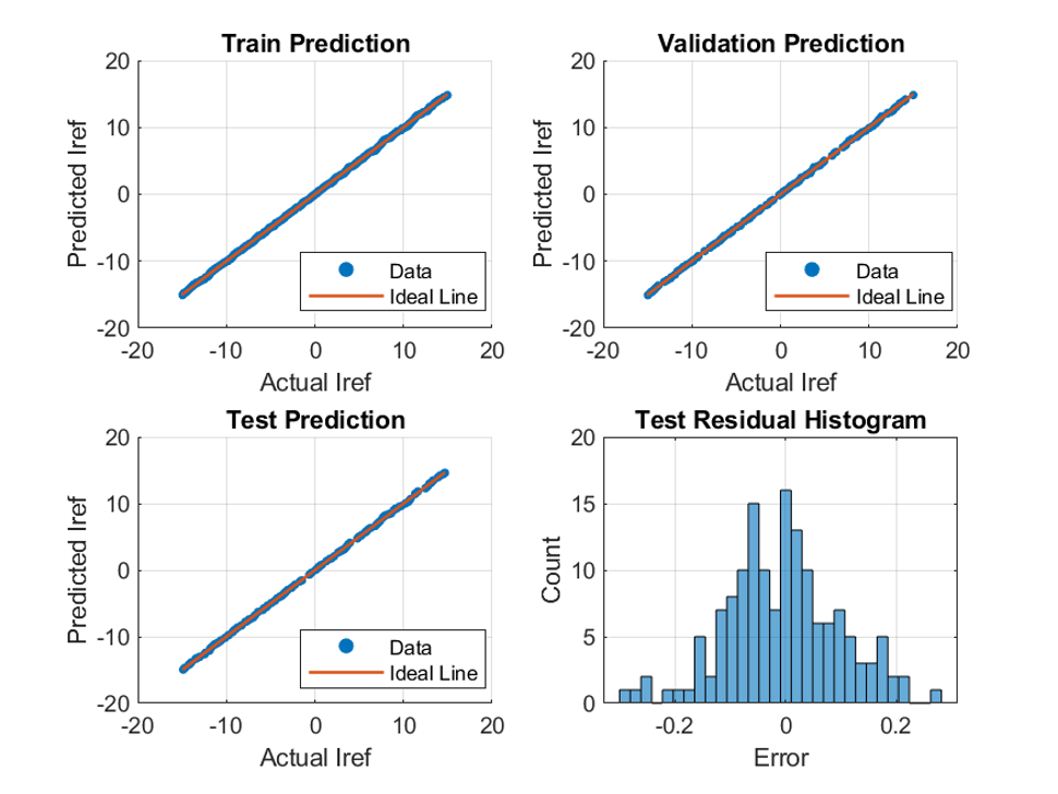
Fig. 8. EMS training, validation, and testing predictions together with the test residual histogram.

Fig. 9. EMS membership functions and nonlinear SOC-P_PV-to-I_ref response surface.

Fig. 10. Distribution of the EMS dataset over battery SOC, PV power, and current-reference target.

Fig. 11. EMS RMSE/MAE comparison and residual sequences for training, validation, and testing subsets.
F. Grid Synchronization, Current Regulation, and LCL Filter
The grid-side controller uses a synchronized orthogonal-reference representation followed by stationary-to-rotating and rotating-to-stationary transformations. For orthogonal components,
[x_d x_q]^T = [[cos(theta_g), sin(theta_g)],[-sin(theta_g), cos(theta_g)]] [x_alpha x_beta]^T | (27) |
The direct-axis current command is associated with active-power exchange, while the quadrature-axis command is maintained near zero for near-unity-power-factor operation. The current errors are
e_d = i_d* - i_d, e_q = i_q* - i_q | (28) |
A PI/PID-form current controller can be represented by
u_d = K_pd e_d + K_id integral e_d dt | (29) |
u_q = K_pq e_q + K_iq integral e_q dt | (30) |
Inverse transformation generates the modulation reference for the PWM bridge. For a single-phase orthogonal representation, average real and reactive powers may be obtained as
P_g = 0.5 (v_alpha i_alpha + v_beta i_beta) | (31) |
Q_g = 0.5 (v_beta i_alpha - v_alpha i_beta) | (32) |
The LCL-type interface dynamics are
L_1 di_1/dt = v_inv - v_c - R_1 i_1 | (33) |
C_f dv_c/dt = i_1 - i_g | (34) |
L_2 di_g/dt = v_c - v_g - R_2 i_g | (35) |
These equations explain the separation between inverter current and grid current visible in the simulation and the attenuation of PWM-frequency ripple before utility injection.
G. Validation Metrics
For N voltage samples with measured/target values y_k and ANFIS predictions yhat_k,
RMSE = sqrt[(1/N) sum_k (y_k - yhat_k)^2] | (36) |
MAE = (1/N) sum_k |y_k - yhat_k| | (37) |
MSE = (1/N) sum_k (y_k - yhat_k)^2 | (38) |
R^2 = 1 - [sum_k (y_k - yhat_k)^2] / [sum_k (y_k - ybar)^2] | (39) |
IV. SIMULATION RESULTS AND DISCUSSION
A. ANFIS MPPT Dataset and Prediction Accuracy
The PV-voltage learning dataset contains 1000 operating points spanning irradiance from 0.7644 to 998.4136 W/m^2, temperature from approximately 15.0023 to 34.9704 °C, and MPP voltage from 216.1666 to 275.1140 V. The mean irradiance, temperature, and PV voltage are approximately 519.15 W/m^2, 24.99 °C, and 245.63 V, respectively. Fig. 2 shows that the dataset covers the irradiance-temperature region rather than concentrating on a single operating line, which is important because the ANFIS must interpolate in two dimensions.
The learned response in Fig. 3 closely overlays the target voltage throughout training and testing. Fig. 4 further shows an almost perfectly linear predicted-versus-actual relationship while retaining a smooth nonlinear surface versus irradiance and temperature. For the 150 reported test samples, irradiance ranges from approximately 5.24 to 985.44 W/m^2 and temperature from 15.00 to 34.88 °C. The actual MPP voltage spans 216.4386-275.1140 V, whereas the predicted range is 216.4388-275.1137 V.
TABLE IIIQUANTITATIVE ANFIS MPPT TEST PERFORMANCE
Metric | Value |
Test samples | 150 |
RMSE | 2.080205 × 10^-4 V |
MAE | 1.560149 × 10^-4 V |
MSE | 4.327253 × 10^-8 V^2 |
R^2 | 0.99999999984 |
Maximum absolute error | 0.001066 V |
Mean signed error | -1.2415 × 10^-5 V |
The RMSE is only 0.208 mV and the maximum absolute error is approximately 1.066 mV over a voltage range exceeding 58 V. This confirms that the trained ANFIS effectively reproduces the target mapping within the sampled operating domain. The very high R^2 should, however, be interpreted as interpolation accuracy for the generated PV-voltage relationship rather than evidence of universal generalization to every PV technology. Experimental validation with sensor noise, aging, partial shading, and parameter mismatch remains necessary before making such a claim.
B. EMS ANFIS Learning Behavior
The EMS result set uses battery SOC and PV power as supervisory variables and grid-current reference as the target. Fig. 7 shows training and checking errors that decrease and then remain bounded over the training process, with adaptive step-size adjustment. Fig. 8 demonstrates that predicted I_ref follows the ideal line over approximately -15 to +15 A for training, validation, and testing data.
The plotted error comparison in Fig. 11 gives approximately 0.092, 0.090, and 0.101 A RMSE for training, validation, and testing, respectively. The corresponding MAE values are approximately 0.073, 0.069, and 0.079 A. Test residuals are concentrated around zero and remain mainly inside approximately ±0.3 A. The close train-validation-test error levels are important because they indicate that the learned EMS surface is not merely reproducing the training samples.
The dataset traces in Fig. 10 contain roughly 700 training observations and 150 observations each for validation and testing, consistent with a 70%/15%/15% partition of the 1000-sample set. The output surface in Fig. 9 varies continuously with both PV power and SOC, avoiding abrupt rule-boundary discontinuities in the grid-current command.
C. Dynamic PV Response Under Irradiance Changes
The system is subjected to five irradiance levels,
G(t) = 1000 (0-0.4 s), 500 (0.4-0.8 s), 300 (0.8-1.2 s), 200 (1.2-1.6 s), 100 (1.6-1.8 s) W/m^2 | (40) |
Fig. 12 shows the corresponding PV voltage, current, power, and irradiance. The PV voltage is maintained near 250 V during the complete sequence, apart from short switching and transition disturbances. At 1000 W/m^2, PV current is approximately 8 A and power is about 2.0 kW. At 500 W/m^2, current falls to approximately 4 A and power to about 1.0 kW. Subsequent 300, 200, and 100 W/m^2 plateaus yield roughly 0.6, 0.4, and 0.2 kW, respectively.
This near-proportional decrease in power with irradiance is expected at fixed temperature, while the maintained voltage indicates that the boost converter continues operating near the ANFIS-predicted voltage reference. The strongest voltage disturbance occurs at the first major irradiance transition at t = 0.4 s; recovery is rapid relative to the 0.4-s duration of each operating interval.

Fig. 12. PV voltage, current, output power, and irradiance during the five-level solar profile.
D. DC-Link Regulation
Fig. 15 shows the DC-link startup and grid waveforms. The DC bus rises rapidly from its initial condition, reaches approximately 300 V almost immediately after energization, and then approaches the 500-V reference through the storage/converter voltage loops. From the plotted response, the bus enters a narrow neighborhood of 500 V by approximately 0.4 s. Any overshoot is visually small, on the order of only a few volts, corresponding to less than approximately 2% of the reference.
After regulation is established, the 500-V bus remains essentially constant despite four subsequent irradiance reductions. This is an important system-level result: PV power changes by roughly an order of magnitude, from 2.0 to 0.2 kW, while the common DC bus remains regulated because the stationary battery and grid compensate for the renewable-power deficit.
The waveform therefore demonstrates empirical closed-loop boundedness and disturbance recovery over the simulated operating sequence. It should not be interpreted as a formal small-signal stability proof because eigenvalues, impedance ratios, gain/phase margins, and LCL resonance damping margins are not evaluated in the available simulation results.
E. Stationary-BESS Response
Fig. 13 shows the stationary battery at an initial SOC of about 25%. The battery voltage rapidly reaches approximately 250-260 V and remains nearly constant. Its discharge current rises to approximately 17 A during the high-power initial interval, corresponding to about 4.2-4.4 kW. After the irradiance reduction at 0.4 s, the current settles near 15 A and then gradually decreases toward approximately 13 A by the end of the simulation. Stationary-battery power follows the same trend, falling from roughly 4.3 kW to about 3.3 kW.
The positive stationary-battery current and power indicate discharge into the common DC link. Accordingly, SOC decreases monotonically from approximately 25.000% to about 24.98% over 1.8 s. The small numerical SOC change is expected because the simulation interval is short relative to the energy capacity of an EV-scale battery, while the power flow itself is several kilowatts.

Fig. 13. Stationary-BESS terminal voltage, current, power, and SOC.
F. EV Battery Charging Performance
Fig. 14 confirms continuous EV charging throughout the solar transitions. The EV battery voltage is maintained near 250 V after startup. Charging current reaches approximately -22 A during the initial interval and slowly relaxes toward approximately -19 to -20 A by 1.8 s. The associated EV-battery power is approximately -5.5 kW initially and about -4.8 to -5.0 kW at the end of the simulation.
With the adopted sign convention, negative EV-battery power represents power absorbed by the battery. The SOC therefore increases monotonically from 9.0% to approximately 9.15%. The key point is that no charging interruption occurs when irradiance falls from 1000 to 100 W/m^2. Instead, the supervisory control shifts the required balance toward the utility while the stationary battery continues to support the DC link.

Fig. 14. EV-battery voltage, charging current, charging power, and SOC.
G. Grid-Side Power Reversal and Reactive-Power Behavior
The grid real and reactive powers are shown in Fig. 16. After the startup transient, the station exports approximately 0.6 kW during the high-irradiance interval between roughly 0.1 and 0.4 s. At the 0.4-s irradiance reduction, the real-power direction reverses and the grid supplies approximately 0.95 kW. The imported real power then rises to about 1.2 kW at 0.8 s, 1.35 kW at 1.2 s, and 1.55 kW after 1.6 s.
This progression directly demonstrates the EMS objective. Lower PV availability does not force a discontinuous EV charging reduction; instead, the grid-current command is increased so the utility progressively supplies the missing power. The transition from negative to positive grid power also confirms bidirectional station-grid interaction.
Reactive power exhibits short transient excursions at startup and irradiance changes but settles close to approximately -0.1 kvar. At the final operating point,
PF ≈ 1550 / sqrt(1550^2 + 100^2) ≈ 0.998 | (41) |
Thus, after the transient intervals, the grid-side operation is close to unity power factor. The current waveforms in Fig. 15 are approximately sinusoidal once the startup transient decays. A numerical THD value is not reported because an FFT-based harmonic measurement is not included in the available result set; claiming a specific THD from the time-domain figure alone would not be technically justified.

Fig. 15. DC-bus voltage, utility voltage, grid current, and inverter-side current.

Fig. 16. Utility-grid real and reactive powers during solar-power transitions.
H. System-Level Power-Balance Interpretation
The result set is mutually consistent across the PV, BESS, EV, and grid plots. During the high-irradiance interval, the PV supplies approximately 2.0 kW and the stationary BESS supplies about 4.3 kW, while approximately 0.6 kW is exported to the grid. The remaining power is of the same order as the roughly 5.5-kW EV charging demand plus conversion losses.
At the lowest irradiance level, the PV contribution is only about 0.2 kW, the stationary BESS provides roughly 3.3 kW, and the grid imports approximately 1.55 kW. Their combined input is close to the approximately 4.8-5.0-kW EV charging power, with the remaining difference attributable to converter/filter losses, DC-link dynamics, and graphical read-off uncertainty. This consistency supports the validity of the control logic and the sign convention adopted in (23).
TABLE IVAPPROXIMATE DYNAMIC OPERATING POINTS READ FROM THE SIMULATION WAVEFORMS
G (W/m^2) | P_PV (kW) | P_g (kW) | BESS (kW) | EV charge (kW) |
1000 | 2.0 | -0.6 export | 4.2-4.4 | 5.4-5.5 |
500 | 1.0 | +0.95 import | ≈3.9-4.0 | ≈5.4 |
300 | 0.6 | +1.2 import | ≈3.6-3.8 | ≈5.2 |
200 | 0.4 | +1.35 import | ≈3.4-3.6 | ≈5.0 |
100 | 0.2 | +1.55 import | ≈3.3 | 4.8-5.0 |
The combined results validate three distinct layers of the design. First, the ANFIS MPPT reproduces the MPP-voltage target with sub-millivolt statistical error over the test set. Second, the converter-level control maintains the PV operating voltage and 500-V DC link despite large irradiance variations. Third, the supervisory ANFIS EMS changes grid-current demand so that EV charging remains continuous while the station transitions from grid export to increasing grid import.
V. CONCLUSION AND FUTURE SCOPE
A dual-ANFIS PV-grid EV charging station has been modeled and evaluated in MATLAB/Simulink. The architecture combines an ANFIS voltage-reference MPPT, PV boost converter, 500-V common DC link, stationary BESS, bidirectional EV battery interface, ANFIS supervisory EMS, and synchronized grid-current-controlled inverter. The MPPT ANFIS uses two inputs, three generalized-bell membership functions per input, and nine first-order Sugeno rules. Across 150 test samples, it achieves an RMSE of 2.0802×10^-4 V, MAE of 1.5601×10^-4 V, maximum absolute error of 1.066 mV, and R^2 = 0.99999999984.
Dynamic simulation further verifies coordinated station operation. The 500-V DC bus settles to its reference by approximately 0.4 s and remains regulated as irradiance decreases from 1000 to 100 W/m^2. PV power correspondingly falls from approximately 2.0 to 0.2 kW. The EMS compensates by reversing grid real power from roughly 0.6-kW export to progressively larger import, reaching approximately 1.55 kW. Simultaneously, the stationary BESS supplies about 3.3-4.4 kW and the EV remains continuously charged at approximately 4.8-5.5 kW, increasing EV SOC from 9.0% to around 9.15%. Reactive power settles near -0.1 kvar and the final operating point corresponds to a power factor of approximately 0.998.
Future work should first implement the controller on a real-time HIL platform such as an FPGA/DSP or real-time simulator to evaluate sampling delay, switch dead time, measurement noise, PWM nonidealities, and communication latency. Second, the EMS should be extended with battery temperature, current/SOC constraints, degradation cost, forecast uncertainty, electricity tariffs, and explicit battery-health objectives. Third, experimental grid-interface validation should include FFT-based current THD, LCL resonance damping, formal small-signal/impedance stability assessment, protection behavior, and laboratory verification of import/export transitions under rapidly varying irradiance and EV demand.
REFERENCES
[1] J.-S. R. Jang, "ANFIS: Adaptive-network-based fuzzy inference system," IEEE Trans. Syst., Man, Cybern., vol. 23, no. 3, pp. 665-685, May/Jun. 1993, doi: 10.1109/21.256541.
[2] H. Abu-Rub, A. Iqbal, and S. M. Ahmed, "Adaptive neuro-fuzzy inference system-based maximum power point tracking of solar PV modules for fast varying solar radiations," Int. J. Sustain. Energy, vol. 31, no. 6, pp. 383-398, Dec. 2012, doi: 10.1080/1478646X.2011.587517.
[3] N. Priyadarshi, S. Padmanaban, J. B. Holm-Nielsen, F. Blaabjerg, and M. S. Bhaskar, "An experimental estimation of hybrid ANFIS-PSO-based MPPT for PV grid integration under fluctuating sun irradiance," IEEE Syst. J., vol. 14, no. 1, pp. 1218-1229, Mar. 2020, doi: 10.1109/JSYST.2019.2949083.
[4] M. G. Villalva, J. R. Gazoli, and E. Ruppert Filho, "Comprehensive approach to modeling and simulation of photovoltaic arrays," IEEE Trans. Power Electron., vol. 24, no. 5, pp. 1198-1208, May 2009, doi: 10.1109/TPEL.2009.2013862.
[5] F. Blaabjerg, R. Teodorescu, M. Liserre, and A. V. Timbus, "Overview of control and grid synchronization for distributed power generation systems," IEEE Trans. Ind. Electron., vol. 53, no. 5, pp. 1398-1409, Oct. 2006, doi: 10.1109/TIE.2006.881997.
[6] M. A. H. Rafi and J. Bauman, "A comprehensive review of DC fast-charging stations with energy storage: Architectures, power converters, and analysis," IEEE Trans. Transp. Electrific., vol. 7, no. 2, pp. 345-368, Jun. 2021, doi: 10.1109/TTE.2020.3015743.
[7] M. M. Mahfouz and M. R. Iravani, "Grid-integration of battery-enabled DC fast charging station for electric vehicles," IEEE Trans. Energy Convers., vol. 35, no. 1, pp. 375-385, Mar. 2020, doi: 10.1109/TEC.2019.2945293.
[8] K. Chaudhari, A. Ukil, K. Nandha Kumar, U. Manandhar, and S. K. Kollimalla, "Hybrid optimization for economic deployment of ESS in PV-integrated EV charging stations," IEEE Trans. Ind. Informat., vol. 14, no. 1, pp. 106-116, Jan. 2018, doi: 10.1109/TII.2017.2713481.
[9] Q. Yan, B. Zhang, and M. Kezunovic, "Optimized operational cost reduction for an EV charging station integrated with battery energy storage and PV generation," IEEE Trans. Smart Grid, vol. 10, no. 2, pp. 2096-2106, Mar. 2019, doi: 10.1109/TSG.2017.2788440.
[10] A. R. Bhatti and Z. Salam, "A rule-based energy management scheme for uninterrupted electric vehicles charging at constant price using photovoltaic-grid system," Renew. Energy, vol. 125, pp. 384-400, Sep. 2018, doi: 10.1016/j.renene.2018.02.126.
[11] J. Engelhardt, J. M. Zepter, T. Gabderakhmanova, and M. Marinelli, "Energy management of a multi-battery system for renewable-based high power EV charging," eTransportation, vol. 14, Art. no. 100198, Nov. 2022, doi: 10.1016/j.etran.2022.100198.
[12] M. Khalid and B. K. Panigrahi, "Decentralized power management in multi BESS-PV based charging infrastructure for EV with SoC balancing," IEEE Trans. Ind. Appl., vol. 59, no. 6, pp. 7392-7403, Nov./Dec. 2023, doi: 10.1109/TIA.2023.3305318.



Comments